What are Diffusion Language Models?

Preface

Dear Reader, I feel like writing this blog for a long time. Diffusion model for language generation is an exciting and emerging field that receives increasing attention. However, up until the moment I am writing this blog, there isn’t a comprehensive guide/intro covering such topics for the members of NLP/ML community who wish to conduct research in this area, prospectively. In this blog, we will walk through the history of diffusion language model, different paradigms in implementation, possible future research directions and applications (also a few of my personal opinion, which might be biased, in italics). The blog will be updated constantly, and I will probably turn this into a survey paper when the time is right.

This blog targets audience who already has sufficient knowledge in Diffusion Models, and traditional autoregressive LLMs. If you don’t, no worries, here are resources I found extremely helpful.

• For Diffusion Models:
  • What are Diffusion Models? by Lilian Weng Strongly recommended
  • Understanding Diffusion Models: A Unified Perspective by Calvin Luo
• For Autoregressive LLMs:
  • Stanford CS224N GOAT course

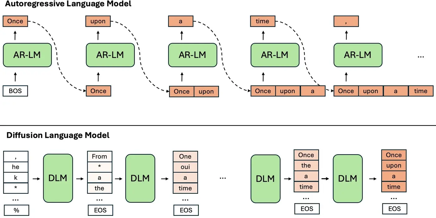
What’s diffusion language model (DLM)?

A brief recap on all the trending autoregressive language model (AR-LM) nowadays, from GPT-2, Llama, to Gemini, ChatGPT, and Claude, these models are using transformer as the common backbone for auoregressive decoding (AR), that is predicting token by token in an left-to-right fashion. By contrast, diffusion language model (DLM) is iteratively refines and predicts the entire sequence from a sampled noisy input as non-autoregressive decoding (NAR). A straightforward (simplified) demonstration of the difference between two paradigms can be shown in the pipeline figure below.

Putting it into mathematical term is, given a sequence we want to predict, \(\mathbf{x} = \{x_1, x_2, \ldots x_N\}\) , AR-LM with parameter \(\theta\) models the following distribution. \(\begin{equation} \label{eq:AR-LM} P(\mathbf{x}; \theta) = \prod_{t=1}^{N} P(x_n | \mathbf{x}_{<n}; \theta) \end{equation}\)

Where DLM take a holistic view of the entire sequence, it models the following distribution, where \(t\) is the timestep in reverse diffusion process (we will get to the details very soon). A larger \(t\) means noiser sequence, closer to sampled from a standard gaussian noise. Consider we are having a very messy paragraph in the beginning and iteratively refines into the passage we want.

\[\begin{equation} \label{eq:DLM} \mathbf{x}_{t-1} \sim p_{\theta}(\mathbf{x}_{t-1} | \mathbf{x}_t, t) \end{equation}\]

Why we need DLM (or NAR)? What’s wrong with AR?

Autoregressive model is extremely successful nowadays, so why do we still need another paradigm? What makes DLM a field worth looking into? Well here are some arguments for you to consider.

• Inherent Disadvantage of AR-LM
  • Error Propagation For autoregressive models, if you made mistake in predicting the current token, there is no chance for going back for revision. Future predictions are always based on this flawed prediction, propagating and accumulating such errors. We call such struggle as error propagation.
  • Indirect Generation Control Current strategies for AR controlled generation depends on extensive training or hacks in decoding strategy. Such techniques are often indirect and inconvienient for users to control the generation. For example, if you want to generate a passage with certain length, you need to train a length predictor or use heuristics like top-k sampling to control the generation. And what’s more, there is no guarantee 😥.
• (Potential) Advantage of DLM
  • NAR As sequence are generated holistically, you can fix and correct previous mistakes and refine the sequence as a whole.
  • Controllability Diffusion models are known to provide simple, training efficient style controlls using either classifier free guidance or classifier based guidance. Such controllability can be easily extended to DLM, where we can control the style of generation using the same techniques (Prafulla et al., 2021, Radford et al., 2021). We can also take this a step further to even more fine-grained controles in lengths, specific text editing, infillings because the model works on the whole sequence representation iteratively (Li et al, 2022, Nie et al., 2025,). This may also extends to tasks with stronger structural constraints (e.g., code, table).
  • Diversity Can produce more diverse outputs compared to beam search in AR. You just need to sample different initial noise.
  • Speed Up Poential for faster generation as stops could be paralleilized, as tokens are generated all-together, instead of waiting for previous outputs iteratively.

Diffusion Model Recap

Diffusion models are very successful and widely adopted in computer vision tasks, such as image generation, super-resolution, and inpainting. The core idea of diffusion models is to learn a generative model by reversing a diffusion process that gradually adds noise to the data. Using the famous DDPM as an example, given a data sample from a real data distribution \(\mathbf{x}_0 \sim \mathcal{D}(x)\), we use a forward process to gradually perturb the data with small amounts of Gaussian noise over \(T\) steps:

\(\begin{equation} q(\mathbf{x}_t | \mathbf{x}_{t-1}) = \mathcal{N}(\mathbf{x}_t; \sqrt{1 - \beta_t} \mathbf{x}_{t-1}, \beta_t \mathbf{I}) \end{equation}\) \(\begin{equation} q(\mathbf{x}_{1:T} | \mathbf{x}_0) = \prod_{t=1}^T q(\mathbf{x}_t | \mathbf{x}_{t-1}) \end{equation}\)

where \(\beta_t \in (0, 1)\) is a variance schedule that controls the amount of noise added at each step. As \(T \to \infty\), \(\mathbf{x}_T\) approaches a sample from a standard Gaussian distribution:

\[\begin{equation} \lim_{T \to \infty} \mathbf{x}_T \approx \mathcal{N}(0, \mathbf{I}) \end{equation}\]

The reverse process then learns to gradually denoise the data, starting from pure noise \(\mathbf{x}_T \sim \mathcal{N}(0, \mathbf{I})\) and working backwards, where \(\mu_\theta\) and \(\Sigma_\theta\) are learned by a fancy neural network model. Again, if you are not comfortable with these concepts, please refer to Lilian’s amazing blog.

\[\begin{equation} p_\theta(\mathbf{x}_{0:T}) = p(\mathbf{x}_T) \prod_{t=1}^T p_\theta(\mathbf{x}_{t-1} | \mathbf{x}_t) \end{equation}\] \[\begin{equation} p_\theta(\mathbf{x}_{t-1} | \mathbf{x}_t) = \mathcal{N}(\mathbf{x}_{t-1}; \mu_\theta(\mathbf{x}_t, t), \Sigma_\theta(\mathbf{x}_t, t)) \end{equation}\]

What’s the fundamental challenge?

Well, if the Diffusion Model is well-established and it has all these exciting perks, why this is not as trending as in the field of computer vision? Good spot, now it comes to the fundamental challenge, the discrepancy between traditional continuous diffusion models, which achieved great success in image generation (such as with Denoising Diffusion Probabilistic Models - Ho et al., 2020), and the domain of discrete text.

Think about an image. It’s made of pixels, and each pixel has colour values (like RGB) that are essentially numbers on a continuous scale. Adding “noise” is intuitive: you can slightly perturb these numerical values, typically by adding small random numbers drawn from a Gaussian (bell curve) distribution. Gradually adding more noise smoothly transitions the image to random static. The reverse process involves training a model to predict and subtract that small amount of noise at each step, gradually recovering the image.

Now, consider text. Language is composed of discrete units – words or tokens selected from a finite vocabulary (e.g., “cat”, “dog”, “runs”). You can’t simply add “0.1 Gaussian noise” to the word “cat” and get something meaningful that’s slightly different but still related in a smooth, continuous way. Applying the original continuous noise formulation directly just doesn’t work.

This discrete nature of text is the core hurdle that requires specific adaptations. How do you define a “forward process” that gradually corrupts text into noise, and critically, a “reverse process” that a model can learn to invert step-by-step?

Researchers have developed clever workarounds to bridge this gap:

1. Operating on Continuous Variables: One approach is to work not with the tokens themselves, but with their continuous variables. Traditional langauge models gives well-constructed word embedding and hidden outputs representations. We could leverage these representations to define a continuous forward process, where the model learns to predict the noise added to these continuous representations at each step. This is similar to how diffusion models operate in the image domain, where the forward process is defined in the latent space of a VAE or similar architecture.
   • Word Embedding (Token Level) Noise can be added to these word embedding vectors, a technique used in models like Diffusion-LM, and the pre-trained DLM GENIE. However, mapping potentially noisy embeddings back to specific discrete tokens at each step introduces its own complexities.
   • Higher Level Latent Representations Works like PLANNER and LD4LG are operating on a higher level latent representations of paragraphs of texts. However, the latent representations are fragile when perturbed by noise, resulting in abrupt semantic changes in reverse diffusion process. My own paper SLD attempts to mitigate this issue cleverly by text-segementation and improved representation learning techniques. Meta’s Large Concept Model is probably the ultimate form of pre-trained DLM following this path.
2. Discrete Corruption Surrogate: More commonly, diffusion models for text define analogous discrete “noising” or “corruption” processes, as explored in papers like . Instead of adding mathematical noise, the forward process might involve:
   • Masking: Randomly replacing tokens with a special [MASK] token, with the number of masked tokens increasing over diffusion steps. The recent trending work of LLaDA, is the pre-trained DLM (8B parameters, largest of all kinds) following this path.
   • Token Substitution: Randomly replacing tokens with other tokens from the vocabulary.
   • Hybrids: Combining these or other discrete corruption methods.
3. Discrete Diffusion: Now a few bold geniuses are thinking, “Hey, if tokens are discrete, why not make the diffusion process discrete as well?”. So we have discrete diffusion over categorical supports. Eminel et al, 2021 introduces extensions of diffusion for categorical data such as language. We model each token as a probability mass vector distributing over \(p \in \mathbb{R}^{V}\), where \(V\) is the size of the vocabulary and use transition matrices \(\mathbf{Q}\) to model transitions between denoising timestops, for example \(q(\mathbf{x}_t |\mathbf{x}_{t-1}) = Categorical(\mathbf{x}_t; \mathbf{p}=\mathbf{x}_{t-1}\mathbf{Q}_t)\). Models like D3PM, and SEDD (ICML 2024 Best Paper) follows this path.
4. 🔥🖼️👊 The Maverick–Text in Image: “Discrete text? What text? It’s an image!” I personally wish you to checkout this GlyphDiffusion. Instead of dealing with the discrepancy, they bypassed by rendering the target text as a glyph image containing visual language content 🤣.

The reverse process then becomes about learning to undo this specific type of discrete corruption. For instance, the model learns to predict the original tokens at the [MASK] positions or identify and correct a randomly sampled variable into meaningful tokens , iteratively refining the sequence from a highly corrupted state back to coherent text. So, while the core idea of diffusion (iterative refinement from noise) remains, the mechanisms for the forward (corruption) and reverse (denoising) processes have to be specifically adapted for the discrete world of language.

Now I will select the representative work of each of these methods to further explain the concept of DLM.

Embedding-Level diffusion – where it begins

As far as I know, Diffusion-LM is probably the first, influencial work that starts the era of DLM. Now suppose we have a sequence of words \(\mathbf{w} = \{w_1, w_2, \ldots, w_n\}\), an embedding fucntion is defined to map each word to a word vector \(Emb(w_i) \in \mathbb{R}^{d}\). So the entire sequence weill be encoded into \(\mathbf{x}_0 = Emb(\mathbf{w}) \in \mathbb{R}^{d}\). So yeah! There we go, we have a continuous space where we can run the conventional diffusion models. We use the typical simplified KL-divergence term in evidence lower bound (which I will not reiterate here) to derive a loss function.

\[\begin{equation} \mathcal{L}_{simple}(\mathbf{x}_0) = \Sigma_{t=1}^T \underset{q(\mathbf{x}_t | \mathbf{x}_0)}{\mathbb{E}} ||\mu(\mathbf{x}_t, t) - \hat{\mu}(\mathbf{x}_t, \mathbf{x}_0)||^2 \end{equation}\]

But don’t forget, we need to convert the embedding back to discrete tokens, you will say this is easy, let’s just have another function transform them back to tokens. Indeed, that’s how it’s done. In Li’s implementation, they model theses steps into the diffusion process as an extra timestep. As shown in the figure below, the forward process consists of an additional Markov transition to obtain the embeddings parametrized by \(q_{\phi}(\mathbf{x}_0 | \mathbf{w}) = \mathcal{N}(Emb(\mathbf{w}); \sigma_{0} I)\) . Then in the reverse process you will have an additional trainble rounding step, parameterized by \(p_{\theta}(\mathbf{w} | \mathbf{x}_0) = \prod_{i=1}^n p_{\theta}(w_i | x_i)\) , where \(p_{\theta}(w_i | x_i)\) is a simple softmax distribution.

Then we can adjust the loss function accordingly. For end-to-end training, we will have the final loss function as below. During the reverse process, you run the inferece by sampling a random embedding sequence containing \(n\) token embeddings (fixed, the same as in the training process) and gradually remove the noise.

\[\begin{equation} \mathcal{L}_{simple}^{e2e}(\mathbf{w}) = \underset{q_{\phi}(\mathbf{x}_{0:T} | \mathbf{w})}{\mathbb{E}} \left[\underbrace{\mathcal{L}_{simple}(\mathbf{x}_0)}_{\text{diffusion Loss}} + ||Emb(\mathbf{w}) - \overbrace{\mu_{\theta}(\mathbf{x}_1, 1)}^{\text{predicted }\mathbf{x}_0}||^2 - \underbrace{\log p_{\theta}(\mathbf{w} | \mathbf{x}_0)}_{\text{rounding}} \right] \end{equation}\]

So, everything seems extremely straightforward right? Or does it? Unfortunately, no 😅. The conversion between continous embedding space and discrete tokens is non-trivial, harder than you think. This rounding is a key challenge in token embedding-level diffusion models. The discretization step can lead to errors that accumulate across the diffusion process, as the embedding space is not uniformly populated with valid tokens. Well isn’t this the notorious data sparsity revisited.

In the paper, there is a major chapter talking about the techniques of how they managed to reduce the rounding error to obtain admissible outputs. For example using reparameterisation trick to make sure every term in the loss models \(\mathbf{x}_0\) explicitly. They also introduce a clamping trick that is maping the predicted vector \(\mathbf{x}_t\) to its nearest word embedding sequence in every reverse diffusion sampling step. Still, a lot of work needs to be done in the future for the sake of generation quality.

Back to the model, with the diffusion pipeline, you can do the fancy conditioning and controlled generation during your inference now. For example, you could have a separate neural network classifier and a class condition \(\mathbf{c}\). During the backward process, you obtain the \(\mathbf{x}_{t-1}\) with respect to the posterior probability using the gradient update below.

\[\begin{equation} \nabla_{\mathbf{x}_{t-1}} \log p(\mathbf{x}_{t-1} | \mathbf{x}_{t}, \mathbf{c}) = \nabla_{\mathbf{x}_{t-1}} \log p(\mathbf{x}_{t-1} | \mathbf{x}_{t}) + \underbrace{\nabla_{\mathbf{x}_{t-1}} \log p(\mathbf{c} | \mathbf{x}_{t-1})}_{\text{classifier guidance}} \end{equation}\]

The paper provides many experiments for controlled generation (e.g., semantics, length, POS and etc.). I want to mention about infilling specifically. That is during the inference process, instead of denoising all the embeddings, some context embeddings are given and fixed (e.g., \(\mathbf{x}_t =\)[w_1] [noise] [w_2]), the diffusion model will mask the gradient of other tokens, only generated the noised token in the middle. However, the other embeddings are used together as conditions naturally during the reverse sampling, as a classifier-free guidance. And you, my clever reader, immediately understands how traditional sequence-to-sequence task can be modelled by giving the input as left contexts only.

GENIE is the first pre-trained DLM (again, as I know) following this token embedding-level diffusion. The model uses continuous paragraph denoise objective for pre-training. The object first applied a hybrid noising techniques to the original text, including token masking (e.g., [w_1] [MASK] [w_2]) and forward diffusion process sampling, then ask the model to recover the clean original text.

Notably, GENIE doesn’t use infilling as the default sequence-to-sequence generation method. Instead, it is using a more Encoder-Decoder approach (yes, like BART or T5), which is another analogues of classifier-free guidance. Similar rounding techniques is applied, they are using an effective KNN algorithm to retreive closets word embedding of each token during reverse sampling and apply rounding to the closest learnt word embedding.